Our goal is to gain skill and comfort in modeling moving objects. Previously, we worked out 4 equations (called the kinematic equations) that are useful in modeling objects that move with constant acceleration. (Yes, it's certainly possible to model motion with non-constant acceleration. You'd either break the motion up into segments, each of which has constant acceleration, which would allow you to use the kinematic equations as we've written them, or you would use calculus to work out different kinematic equations. We won't do this.)
Use of these equations allows us to, in a very real sense, predict the future. Here's a simple example: If I know how fast an airplane is flying, I can predict when it will land at an airport 800 miles away. Here's another example: If a manned rocked leaves Earth for Mars, a NASA engineer can predict exactly when it will reach the red planet, thus determining how much food must be carried along. And while we're talking of space, astronomers can predict the exact date and time of the next solar eclipse.
Before we continue our quest to gain skill at modeling moving objects, let's pause to consider the big picture.
First, realize how remarkable it is that the universe operates in such a way that we can predict the future (in many cases).
Second, realize that predicting the future is easy for simple systems and potentially very difficult (if not logistically impossible) for complex systems. This is why I know that if I drop an apple, it will fall to the ground in less than a second, but I don't know when the next car accident in town will occur.
Third, realize that many complex systems can be approximated by simple systems, allowing us to gain some insight into the system and perhaps arrive at some approximation of its future state. Meteorologists do this when they provide our weekly weather forecast.
Why should YOU bother with modeling the movement of various objects (and later in the course, modeling other aspects of our world)? Well, it "trains your brain" to think in a more-sophisticated, logical manner. It also gives you a new way to think about the world. You are introduced to a modern, scientific viewpoint which was wrestled into existence over hundred of years by many that came before us. And, for many of you, this skill will be necessary in your future career, especially if you become an engineer.
Humans are a visually-oriented sort of animal. "A picture is worth a thousand words," as they say. And thus it's helpful to model motion with pictures, i.e. graphically. If we can model motion both graphically and with mathematical formulas, we can develop a deeper, more intuitive understanding of our models, as well as the world itself.
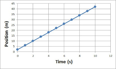
Take a look at the following graph, which illustrates an object moving with constant velocity.


Remember, acceleration is defined as:
a = Δv / t
which is "rise over run" on a velocity vs time graph; i.e. it's the slope of a velocity vs time graph.
Remember, just because the acceleration is toward the east does not mean the car is physically moving eastward. In this case, yes, the car happens to be moving eastward.
It is the velocity which tells you which way the object is actually moving, not the acceleration.
additional resources
practice problems
Δx = vavgt Δx = vit + ½ at2
vf = at + vi vf2 = vi2 + 2aΔx
Δx = vavgt Δx = vit + ½ at2
vf = at + vi vf2 = vi2 + 2aΔx

The standard 4
kinematic equations.


You should think about the equation xf = vavgt + xi until it's clear to you that it's the formula for a straight line (with x on the vertical axis and t on the horizontal axis), in which vavg is the slope of the line and xi is some object's position when time is zero.
And you should think about the equation y = 4x + 2 until it's clear to you that, as it describes an object's motion with time, the 4 must be the object's average velocity and the 2 its starting position, i.e. its position at t = 0.
So, here's how it would actually go down. You collect data on some object, recording its position (relative to some reference point) each second over a period of 10 seconds. You then plot the data and obtain a linear graph. Realizing the graph is linear, you then pick two points (x1, y1) and (x2, y2) and work out the equation of the line, in the form y = mx + b, where m = (y2 - y1) / (x2 - x1). Knowing a bit of physics, you then interpret the "m" -- the 4 in this case -- as the average velocity of your object. And you interpret the "b" -- the 2 in this case -- as the starting position of your object.
If asked to provide a model of your object's motion, you might write: xf = 4t + 2. (Here you are making the choice to use meaningful variables instead of the generic y and x.) And if you wanted to indicate the object's direction (let's pretend like the object is moving north), then you'd write xf = (4 j)t + (2 j).
What can you do with this formula? Well, you can work out exactly where the object was at any given time during those 10 seconds. If we choose a time for which we don't have a data point, within the original range, the process is called interpolation. We can interpolate, for example, the object's position after 5.5 seconds had passed: xf = (4 j)(5.5) + (2 j) = 24 j meters from the reference point.
What was the object's displacement over those 5.5 seconds? Given that displacement Δx = xf - xi, its displacement was 24 j - 2 j = 22 j meters. That is, it moved 22 meters north. (Since it started at the 2-meter mark, it ended at the 24-meter mark.)
We can also, with a bit of justification, extrapolate the data to find the object's position at a time after 10 seconds, assuming the object maintained its constant motion. (From Wikipedia: "Extrapolation is the process of estimating, beyond the original observation range, the value of a variable on the basis of its relationship with another variable.") Look, we're going to predict the future! Where will the object be after a total of 12 seconds?
xf = (4 j)(12) + (2 j) = 50 j meters from the reference point.
The formula that generates this linear graph is of the form y = mx + b, specifically
y = 4x + 2.
This formula is modeling simple motion, and therefore it must be equivalent to one or more of our 4 kinematic equations, which are the equations for modeling simple motion. Careful thought should lead you to Δx = vavgt, which can be rewritten as:
xf = vavg t + xi
y = m x + b

How would you interpret the equation of motion y = 8.2x + 5?
What does a larger slope indicate?
What would a negative slope indicate?
Tom and Jerry (or was it Ben and Jerry?) are racing one another along a straight track. Their positions were measured once each second, and the data has been plotted below.
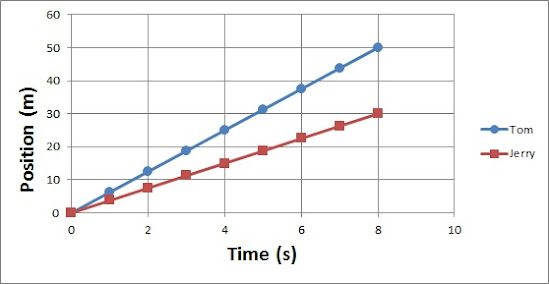
Who ran faster, Tom or Jerry? And how do you know?
About how long did it take Tom to travel 20 meters? About how long did it take Jerry to travel 20 meters?
Yes, Tom ran faster than Jerry. You can tell because his graph has a steeper (or larger) slope, which represents his average velocity. That is, Tom covered more distance per unit of time.
Can you work out the equations of motion for the two? Try it.
Now see if you can interpret the data below. The data pertains to Robert, who began by running north.

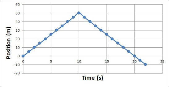
Did you work out that Robert changed directions after having run for 10 seconds?
How did his speed forward (north) compare to his speed backward (south)?
How would you interpret his final position having a negative value (-10 m)?
Could you work out his equation of motion?
Do any of the kinematic equations generate a graph of this shape?
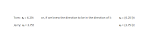
We need an equation for x in terms of t, which rules out the
bottom two equations in the picture at right. The top left equation
is a linear relationship; that can't generate our upside-down-V
graph above. What about the top right equation? Perhaps you
recognize this as a quadratic equation, which it is. It's graph
is curved. So it appears we are not able to model Robert's
motion. What's the problem?
The problem is that Robert does not have a constant acceleration,
and this is a necessary condition for us. The kinematic equations only model constant-acceleration motion. (Please be careful not to confuse constant acceleration with constant velocity. Constant velocity (think speed) is not required. Velocity is allowed to change, but if it changes, it must change by the same amount every second.)
Here's what we can do. We can break up his motion into two segments, each of which has constant acceleration.
During the first 10 seconds, Robert has a constant acceleration of zero. That is, his velocity is unchanging; he is not speeding up or slowing down, just running north at 5 m/s. We could write: vavg = 5 j (m/s).
During the remaining 12 seconds, Robert again has a constant acceleration, and again it is zero. His velocity is again unchanging, although this time it's 5 m/s south. We could write: vavg = - 5 j (m/s).
But right at 10 seconds, his acceleration is NOT zero. His velocity DOES change, from a positive 5 m/s to a negative 5 m/s. And this abrupt acceleration prevents us from modeling the entire 22 seconds with a single equation. (If you think about it, the graph suggests an infinitely large acceleration. The velocity is shown to change from 5 j to -5 j in a time interval of zero seconds. Realize this is not physically possible, and thus our model must be a simplification of what actually happened.)
His equations (plural) of motion could be written as:
xf = (5 j)t, for 0≤t≤10
xf = (-5 j)t + 100 j, for 10≤t≤22
Can you use the equations of motion to determine Robert's displacement at t = 14 seconds? What is his displacement at 5 seconds? What is his total displacement, at t = 22 seconds?
Click here for the answers:
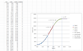
Okay, now take a look at the graph below. The data was collected from a car driving east along a straight country road.
Δx = vavgt Δx = vit + ½ at2
vf = at + vi vf2 = vi2 + 2aΔx

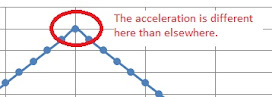
The acceleration is different here than elsewhere.
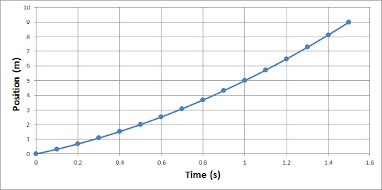
After plotting the points, I asked my computer to generate the equation for this curve.
This is how you ask in Microsoft Excel.
The computer returned the equation: y = 2x2 + 3x
Do you recognize this as a kinematic equation?
If the computer "understood" that you were plotting position versus time, it might return the equation in the format: xf = 2t2 + 3t
y = 3 x + 2 x2
xf = xi + vi t + ½ a t2
The job of the physicist is to interpret correctly the equation provided by the computer. Realize that the 3 tells us the car's initial velocity (okay, so velocity requires an indication of direction, but we were told that motion was east, so to be precise we could say vi = 3 i (m/s); if the car was going west, then the computer would have returned -3 and we'd say vi = -3 i (m/s)).
Continuing onward, the 2 is equal to half of the acceleration, which means the car has an acceleration of 4 m/s/s. And because the 4 is positive, as opposed to negative, we can write a = 4 i (m/s/s). You might think it's strange that a ½ appears in the equation and that 2 is half of the acceleration and not the acceleration, but this model has been proven to accurately model motion and its predictions of the future consistently turn out true. So the ½ stays.
There is no term in our y equation that matches up with xi, which indicates
xi = 0; i.e. the car began its motion from our designated reference point. When modeling read-world motion, you typically force this to be true. That is, you intentionally consider where an object begins its motion to be the origin of your Cartesian coordinate system. Remember, the coordinate system is something you impose onto a situation in order to help you analyze the situation. Impose it in whatever way makes the motion easier to analyze (or the equation easier to work with).
Okay, let's do something with our equation of motion. Let's use it to predict the future by extrapolating. Assuming the car continues to accelerate at 4 i (m/s/s), how far from its starting point will it have traveled after 3.6 seconds?
xf = 2t2 + 3t
xf = (2 i)(3.62) + (3 i)(3.6) = 25.9 i + 10.8 i = 36.7 i (m)
The car traveled 36.7 meters eastward from its starting position.
Taking things a step further, can you use another of the kinematic equations, along with information obtained from the one above, to find the velocity of the car at t = 1.2 seconds? You will be using two models of the car's motion to get what you want. It's a big step forward, but I think you can do it.
Try it before reading on! Remember Roger.


To find the velocity at a time of 1.2 seconds, we need a model (an equation) that contains vf. We have a couple to choose from.
Let's see what we can do with vf = at + vi.
We found earlier, using the equation generated by my computer, that vi = 3 i (m/s) and a = 4 i (m/s2). We can substitute these values into the model vf = at + vi to obtain vf = (4 i)t + 3 i. Evaluating this equation at t = 1.2 s, we get vf = (4 i)(1.2) + 3 i = 7.8 i (m/s). We have our answer: After 1.2 seconds, the car has attained a velocity of 7.8 m/s eastward. Does this make sense? Stop and reflect on what you've done.
Okay, now use one of our models to find the time at which the (instantaneous) velocity is 4.6 m/s eastward.
Afterward, check your answer here:
You might be wondering, could you have found the velocity at t = 1.2 seconds using the other kinematic equation, vf2 = vi2 + 2aΔx? How did I know to pick the shorter of the two equations? Here's my answer:
Yes, you could have used the longer equation. However, I realized that I had what I needed to "plug in" to the shorter equation, and I didn't have a Δx to "plug in" to the longer equation. I could have found Δx at t = 1.2 seconds using the equation of motion given us by the computer, and then I would have had what I needed to use the longer equation, but that would be extra work. It's also the case that the more "problems" you solve, and the longer you do physics, the better your intuition is when it comes to choosing models.
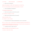
Now I want you to analyze a graph of a different car's motion. This car is heading west. The computer has returned the following equation of motion: y = -5x2 - 2.2x. How much can you work out based on this graph and equation?
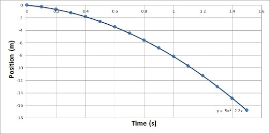
Try to answer the following questions. Use a pencil and paper; don't try to do it in your head.
- What is the car's acceleration?
- Is the car speeding up or slowing down?
- What is the car's position at a time of 0.63 seconds?
- What is the car's velocity at a time of 0.63 seconds?
- How much has the car's velocity increased between t = 0 and t = 0.63 seconds?
- At what time is the car's velocity -50.2 m/s?
After you try these out, check your answers here.
Position vs time is not the only useful graph of an object's motion. It can be quite helpful to look at an object's velocity over some period of time.
If we backtrack to the car driving east on a straight country road, we've already worked out that vf = (4 i)t + 3 i.
Let's graph this equation. vf goes on the vertical axis (we have to resist the temptation to say y-axis) and t goes on the horizontal axis (again, resist the temptation to call this the x-axis).

It shouldn't surprise you that the graph is linear. The velocity is increasing steadily. Every second, the velocity increases by 4 m/s. And it started at 3 m/s.
y = m x + b : generic equation for a linear relationship between y and x
vf = a t + vi : specific equation for a linear relationship between vf and t, using variables
vf = 4 t + 3 : specific equation for a linear relationship between vf and t, with known values substituted
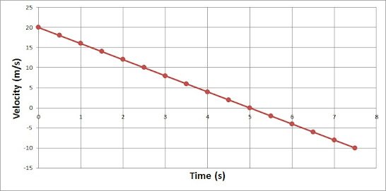
What do you think the velocity graph for the westward traveling car is? (The car for which we obtained
y = -5x2 - 2.2x) Here it is.

If you haven't yet realized it, realize it now: the slope of this particular graph is an acceleration. Here, the slope is -10 m/s2. (Yes, the slope has units, because it refers to the rate at which velocity, which itself has units, is changing.) And the initial velocity is -2.2 m/s. Which makes the equation for this graph: vf = (-10 i)t - 2.2 i.
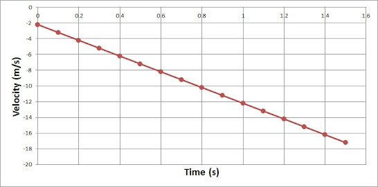
Now take a look at the velocity vs time graph below. Can you make sense of it? What is the object physically doing? Can you work out one or more of the equations of motion for this object, whatever it is?
Try to make sense of this graph before reading on! Seriously.
So, did you realize that this object has a negative acceleration? Did you realize that it changes directions at t = 5 seconds, when it crosses the axis. Prior to 5 seconds, it has a positive velocity (which could mean it's headed either north or east or at least forward), and then past 5 seconds it has a negative velocity (which would mean motion opposite the original direction). Right at 5 seconds, it's momentarily at rest.
This object is slowing down as it moves forward, between 0 and 5 seconds, and then speeding up as it moves backward, between 5 and 7.5 seconds.
As a reminder:
For this graph, between 0 and 5 seconds, a is negative and v is positive, which means the positive velocity is reduced each second, and the object is slowing down as it moves forward. Note that its velocity is approaching zero.
Between 5 and 7.5 seconds, a is negative and v is also negative, which means the negative velocity is becoming more negative, and the object is speeding up heading backwards. Its velocity is moving away from zero.
This motion is similar to that of a ball rolled up a smooth incline. It slows as it moves forward (due to gravity), eventually stopping (for just a moment), and then it rolls back down the hill, gaining speed as it goes.
Before we leave this graph, try to write out both the vf and Δx equations of motion. Then find the displacement of the object at t = 5 seconds. After doing this, check your work:
In everyday language, to accelerate means to "speed up". Not so in physics. Here, to accelerate simply means to change your velocity.
If the direction of the acceleration matches the direction of velocity, the object will "speed up", while if the direction of acceleration is opposite to that of the velocity, the object will "slow down".
While an object always travels in the direction of its velocity, it does NOT always travel in the direction of its acceleration. Specifically, it does not when it's slowing down.

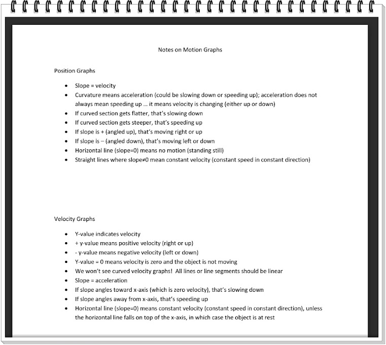
Here are some general rules for interpreting position and velocity graphs.

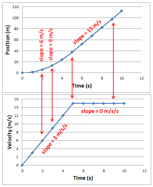
The two graphs at left both correspond to the motion of a car heading east. One graph depicts the car's position with time, and the other graph depicts its velocity with time.
The equation of motion that yields the Position vs Time graph is:
Δx = (1.5 i)t2, 0≤t≤5 (which is a form of Δx = vit + ½ at2, with vi = 0)
Δx = (15 i)t, 5≤t≤10 (which is also a form of Δx = vit + ½ at2, with a = 0)
*Realize the equation gives us Δx, not xf. If you're interested, xf = (1.5 i)t2, 0≤t≤5 and xf = (15 i)t - (37.5 i), 5<t<10.
Don't worry so much about being able to work out these equations from the graph. (Personally, I had access to the underlying data points.) Just spend some time making sense of them, now that I've given them to you.
Can you tell from the two parts of the equation of motion that the acceleration of the car is initially 3.0 m/s2, and then it transitions to 0 m/s2 at 5 seconds?
You can't easily "see" the acceleration on a Position vs Time graph. It's NOT the slope of the curve; the slope is an indication of velocity. Rather, the acceleration is a measure of the rate at which the slope is changing. The best you can really do here is to notice that the slope isn't changing once we pass 5 seconds, so that's when the acceleration must be zero.
However, if you look at the Velocity vs Time graph, the slope (which is the rate at which the velocity is changing with time) is an indication of acceleration. And here, it's easy to see that the acceleration of the car is 3 m/s2 for the first 5 seconds and then 0 m/s2 for the next 5 seconds.
Also, realize that the instantaneous slope at a particular time on a Position graph is equal to the velocity at that instant and is therefore the "y-value" on the Velocity graph, for that particular time. For example, at t = 2 seconds, the slope of the position graph is 6 m/s (you can't tell by looking), and thus on the velocity graph, the velocity takes on the value 6 at that time. (So, how could you have worked out that the slope of the position graph at t = 2 s is 6 m/s? Either by examining the equation of motion corresponding to that graph, or by looking for the "y-value" on the Velocity graph at t = 2 s. You could also use the velocity equation of motion (shown below) to calculate the velocity at any time, including t = 2 s.)
Here are the equations of motion that yield the Velocity vs Time graph.
vf = (3 i)t, 0≤t≤5 (which is a form of vf = at + vi, with vi = 0)
vf = 15 i, 5≤t≤10 (which is also a form of vf = at + vi, with a = 0)
In addition to being able to interpret (and sometimes generate) equations of motion, you also want to be capable of seeing a position graph and then being able to create a quick sketch of the corresponding velocity graph, and vice versa. Be thinking about this as you go forward. This skill will require practice before you're good at it.
For motion with constant acceleration, or at least constant within intervals like above, you won't ever see a curved velocity graph. Why? Because a curved velocity graph indicates that acceleration (which is the slope of the velocity graph) is changing, which contradicts our original premise.
When there is nonzero constant acceleration, the position graph will curve, however. In fact, curvature on this graph is a tell-tale sign of acceleration. And when it comes to the curvature, it is always the smooth curve of a parabola, consistent with our quadratic equation of motion:
Δx = vit + ½ at2.


problems -
creating graphs &
trend lines
*Excel file

problems -
drawing velocity graphs based upon position graphs
-the Physics Classroom website (1-D Kinematics: Lessons 3 & 4)


Download the Wolfram CDF Player to explore these (and many other) interactive demonstrations.
(If you are using a school-issued laptop, you must download the CDF Player through the Software Center.)
*Hieggelke, C. J., Maloney, D. P., & Kanim, S. E. (2012). Newtonian tasks inspired by physics education research: NTIPERs. Boston: Addison-Wesley.

how to plot data and add a trend line in Microsoft Excel


Forces
Kinematics
