Our near-term goal is to model objects moving within (only) 2 dimensions, such that part of the motion is aligned with unit vector i and part with unit vector j.
But first we shall consider something both relevant and very interesting.


Let's imagine a passenger train moving forward at a constant velocity. Inside is a man, standing up, holding his smart phone. Then, tragically, he drops it.
What does the man see?
He sees the phone fall straight downward, landing near his feet.
But what would an observer standing outside of the train, looking in through a window, see?
The phone does not fall straight down; rather, it moves forward, along with the train, as it falls downward.
Below is an illustration of the phone's path, from both points of view (or reference frames). Notice these graphs, unlike those we've worked with before, do not have "time" on the horizontal axis (technically called the abscissa, but I just can't get used to that word). Rather, they show position in 2D space, with each data point separated from the next by 0.05 seconds in time. That is, they're like time-lapse photos, with the phone indicated as a blue dot, and with the photos 0.05 seconds apart.
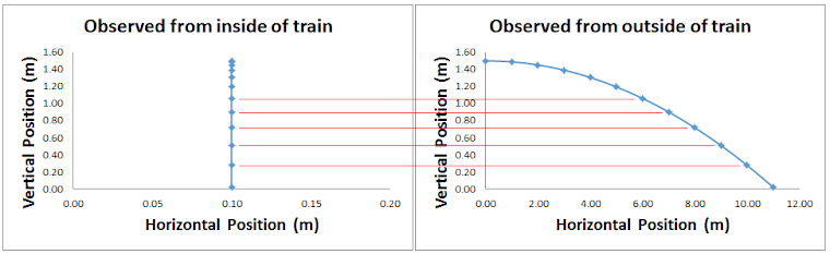
From one point of view, the ball falls straight down. It's path is linear.
From another point of view, the ball moves along a longer curved path. It looks to be a parabola.
This is interesting!
The distance traveled by the phone varies depending on your reference frame! Yet the time it takes for the phone to strike the ground certainly cannot differ; we all hear and see it hit the ground at the same time (ignoring the effects of relativity). This implies that the speed of the ball, too, differs according to one's reference frame. The person standing outside the train sees the ball moving faster than the person inside the train. (Of course he does. To him, not only is the phone falling, it's moving forward at the speed of the train.)
What are we to make of this?
Here's the important take-away. Whether or not the phone appears to be moving forward has no effect on how quickly it moves downward under the influence of gravity. Notice the horizontal red lines drawn on the graphs above. I added them to show that the vertical position of the phone (i.e. its height) is the same regardless of the reference frame, at each point in time. Both observers see the phone falling downward at the same rate. (You know what that rate is, right?)
Here's the take-away, stated differently. For a freely falling object,
horizontal motion and vertical motion are independent of one another.
How quickly an object moves forward while falling has no effect on how quickly the object moves upward or downward. (Again, how could forward speed affect falling speed when, from one point of view, it doesn't even have a forward speed?)
Here's an interesting thought, based upon the previous reasoning.
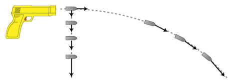
If a bullet is fired from a level gun at the same time that a second bullet is dropped from the height of the barrel, the two bullets will hit the ground at the same time!
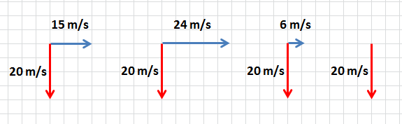
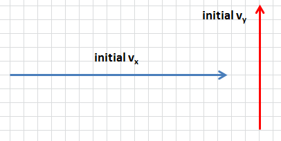
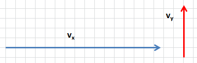
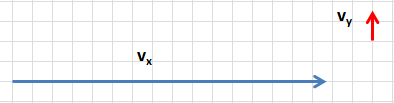
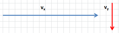
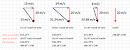
To further emphasize the point being made above, let's take a look at four freely-falling objects. Each object has been falling for two seconds, which accounts for its downward speed of 20 m/s. (We're assuming the local acceleration of gravity is 10 m/s2.) Three of the objects were launched forward and are still traveling forward as they fall, while the fourth object was simply dropped.
The vectors depicted below represent the vertical and horizontal velocities of the four objects. Traditionally, they're called the vertical and horizontal components of the velocity, And the point: the horizontal velocity has no effect on the vertical velocity. All four of these objects will land in different places, if launched from the same spot, but they will all take exactly the same length of time to land.
The independence of the vertical and horizontal velocities is interesting, but is it actually important for our purposes?
Yes! It allows us to model the vertical motion of an object without having to worry about or take account of its horizontal motion, and vice versa.
Now, think about it. Is our first object moving forward at 15 m/s and separately moving downward at 20 m/s, at t = 2 seconds? What I'm showing you is that we can think of it moving that way. But if you point a radar gun at the object, will it register 15 or 20 m/s? No. It will show you the actual speed, which is a combination of the 15 and 20. As the components of the velocity are vectors, we add them as vectors, and they sum to 25 m/s. That's what the radar gun measures.
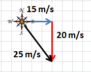
Remember, we add vectors head-to-tail. The sum of the two velocities is the black vector. It represents the actual, measurable velocity of the object. The Pythagorean theorem tells us its value, 25 m/s. Trigonometry allows us to find its direction, 53.13° south of east.
The object is actually moving at 25 m/s, angled downward and to the right. Thinking of that motion as being comprised of two separate and independent velocities, one horizontal and one vertical, is a useful way of thinking of its motion. Its a useful model of what's happening. Make sure you understand this.

Okay, something is bothering me.
If something is falling downward, it is not moving south.
And something moving upward is not moving north.
In the case of the falling object above, I suppose we should be saying its direction is 53.13° below the horizon
A lot of people avoid having to choose the right phrase by simply drawing the vector and labeling the angle.
Okay, you practice now. Add the other pairs of vectors.
(Click on the image for the answers.)
The graphic above illustrates the velocity of a ball, thrown through the air, at six different moments. At each moment shown, the horizontal and vertical components of the velocity are shown, along with their sum (the actual measurable velocity).
Again, we don't directly see the horizontal and vertical velocities as if they were separate from one another. We just see the ball moving along a smooth curve (it's a parabola, by the way; I'll prove this later). But we're physicists trying to model the world. And we've found that it's useful to think about the horizontal and vertical motions as separate from one another. And we can do this because they are independent of one another!
Notice anything interesting in the velocities above? There are at least two interesting and important things you should be able to pick out.
We're making progress analyzing motion in two dimensions. The next step is to look at some data, representative of a ball kicked through the air, although we'll ignore air resistance (a little nod to Galileo). As for the data, we have time in seconds, horizontal position in meters (relative to some start point; the "zero" of our Cartesian coordinate system), and vertical position in meters (also relative to the "zero").

While we're practicing adding velocity components to get the actual velocity, in "the real world" it's usually the other way around.
Normally, you see a ball moving at some speed in some direction, and you "resolve" that motion into components.
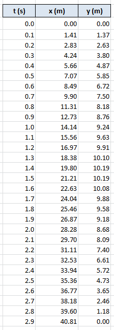


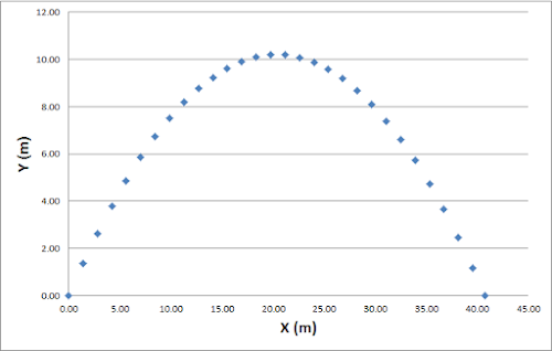
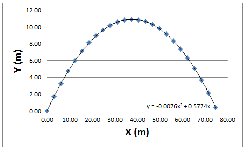
There are three typical ways to plot this data. First, we'll plot the ball's horizontal position (x) against its vertical position (y).
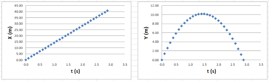
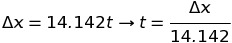
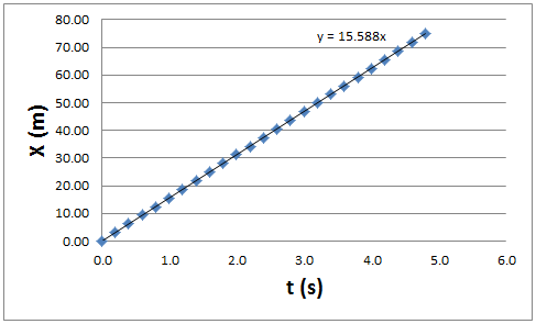
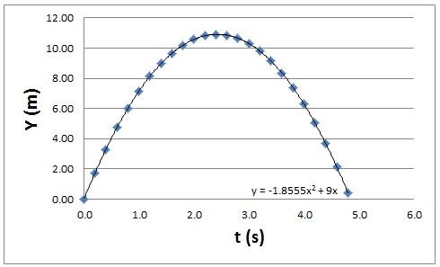
And now we'll plot X vs time and, separately, Y vs time.
We have enough new information to keep us busy for a while. Pay careful attention here.
Thus far, every graph we've created or analyzed has had time on the horizontal axis (except for the two graphs at the top of this page). The Y vs X graph, above, does not, so let's save it for later.
I'vs asked my computer (Microsoft Excel, specifically) for the best-fit line through the data points in X vs t. It returned: y = 14.142x
We've learned how to interpret this. It's actually ∆x = 14.142t, which can be associated with one of our kinematic models. You can interpret our function as ∆x = vavgt, which means that the ball's average velocity in the horizontal direction is 14.142 m/s. You can also interpret our function as ∆x = vit + ½ at2, which means that the ball's initial velocity in the horizontal direction is 14.142 m/s and its acceleration in the horizontal direction is 0.0 m/s/s.
If the ball's initial horizontal velocity is 14.142 m/s, and the ball is not accelerating horizontally, then the horizontal velocity will remain at 14.142 m/s. The ball is always moving forward at that speed. That's why we also find its average horizontal velocity to be the same value. Important Point: Our data supports the hypothesis that the horizontal velocity of a projectile is constant. Turns out, this is true. Stop. Repeat this to yourself. State it in other words.
Now let's look at the Y vs t graph. Again, I've asked my computer to find the equation of the smooth curve that goes through our data points. It returned: y = -4.9x2 + 14.142x
Yes, we know how to interpret this. First, let's rewrite it as ∆x = -4.9t2 + 14.142t ... or is it ∆y = -4.9t2 + 14.142t? Should we use x or y?
Okay, so we need to work out a way to differentiate between horizontal and vertical quantities.
We could state both models (horizontal and vertical) like this:
∆x = (14.142 i)t
∆x = (-4.9 j)t2 + (14.142 j)t
Or we could state them like this:
∆x = 14.142t
∆y = -4.9t2 + 14.142t
Which do you prefer?
Since I prefer the second notation, we'll use it below.
Again, plotting our data resulted in the following two models.
∆x = 14.142t
∆y = -4.9t2 + 14.142t
We've already interpreted the first model as saying that the ball is moving forward at a constant 14.142 m/s.
The second model is obviously ∆x = vit + ½ at2, which tells us that the ball is initially moving vertically (upward) at 14.142 m/s but is accelerating at -9.8 m/s2 (since half of the acceleration is -4.9). The ball's vertical velocity, unlike its horizontal velocity, is not constant. It decreases by 9.8 m/s every second.
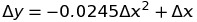
If we algebraically combine our two equations, eliminating t, we obtain the equation for our third and final graph, Y vs X.
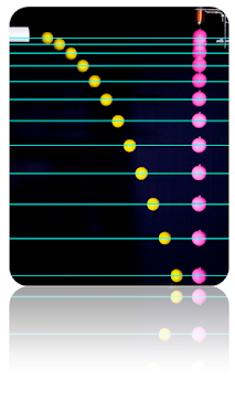
This graph is like a time-lapse photo of the ball, with the photos 0.1 seconds apart.
Yes, it's a parabola. I'll prove it later.

Δx = vavgt Δx = vit + ½ at2
vf = at + vi vf2 = vi2 + 2aΔx

This way is consistent with what we've done in the past. Here, x does not mean horizontal; i does. And j means vertical.
This way leaves out the i and j notation. In a sense, that makes this wrong. But a lot of people choose this notation because it's less cumbersome. And it's less likely you'll confuse horizontal and vertical quantities.
(Personally, I prefer this notation when modeling projectiles.)


This equation is a model of the ball's motion, but it's not one of our 4 standard kinematic equations.
We don't typically use this model. That's because, as we worked out before, horizontal motion and vertical motion are independent of one another, and it's easier to look at them separately (each versus time).
What does the -0.0245 represent? Eh, I don't know. We could probably work it out if we really wanted to.
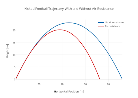
But here's one important thing we can learn from this equation of Y vs X. The actual path of the ball through the sky is parabolic. I told you I would prove it. (Any function y(x) that is a polynomial of degree 2 in x is a parabola with a vertical axis.)
The actual path of a real ball through the air is not exactly a parabola because of air resistance.
We'll ignore air resistance and assume parabolic flight paths for our projectiles.
Mythbusters asks,
"Will a dropped bullet and a fired bullet
really hit the ground at the same time?"
The standard 4
kinematic equations.

In case you were wondering. I asked my computer to give me the equation for the Y vs X data. Surely enough, it gave me this same equation.
A great way to gain insight into projectile motion is to play around with the following simulation, made available by the University of Colorado at Boulder.


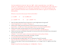
Using the simulation, can you find the answer to these two question?
1) What angle results in the greatest horizontal displacement or range?
2) A 30 degree launch angle results in a certain range. What other unique launch angle achieves the same range? Can you justify, in words, how two launch angles can result in the same range?
We need more practice.
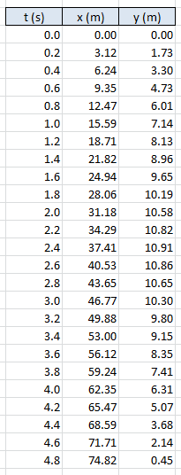
I'm going to show you the position-time data for a new projectile. This one was not launched on Earth, but fortunately our kinematic models are valid throughout the universe. (Did you realize that?)
Glance over the data, then carefully study the graphs. I've had the computer determine the lines of best fit and they are printed on the graphs. (I suppose if the line of best fit isn't straight, I shouldn't call it a "line". Perhaps a best fit curve. But -- and we will cover this later -- plotted data that is not linear can be made linear by changing what is placed on the axes. This is called linearizing the data, and it's very useful in certain situations. Don't worry about it for now.)
I want you to correctly interpret the two functions below. Rewrite them properly, in the format of one of our kinematic models. Actually do this! (Remember Roger?)
No seriously, stop and write down the functions on a piece of paper.
Try to answer the following questions based on your models.
- Was the object launched from the ground or some height above the ground?
- What was its initial horizontal velocity? Did this horizontal velocity change?
- What was its initial vertical velocity? Did this vertical velocity change?
- What was the local acceleration of gravity? Can you use the Internet to determine what planet has this rate of free-fall?
- Did the object accelerate horizontally, vertically, or both?
- At what time did the object land? Hint: It's between 4.8 and 4.9 seconds.
- What was the object's final horizontal displacement, i.e. its range? Hint: It's slightly more than 74.82 m.
Check your answers here after you attempt these questions.
Okay, let's involve some vectors. Below, I've depicted the horizontal and vertical components of the initial velocity. (Initial, of course, means t = 0 s.) The exact length or magnitude of these two vectors are the answers to questions 2 and 3 above.
I want you to add them together to get the initial velocity, both magnitude and direction.
Earlier, you should have answered that the horizontal velocity never changes, while the vertical velocity decreases by -3.711 m/s every second.
Let's redraw our velocity vectors (the components) to represent velocity at time = 1 second.
The horizontal velocity vector has not changed, while the vertical velocity vector is 5.289 m/s in magnitude, which is 3.711 m/s less than the initial value of 9.000 m/s. (You might notice that I'm created a scale where each "box" on the graph paper is 1 m/s wide and 1 m/s tall. I could have chosen a different scale, as long as I was consistent. You can choose whatever scale you want, unless you're told to use a certain one.)
Now we can add these two new vectors to find the velocity of the object at t = 1 second. Please do so! Find both the magnitude and direction of the object's velocity at this moment in time.
Continuing on, let's redraw the velocity vectors at t = 2 seconds.
The horizontal velocity vector has not changed, while the vertical velocity vector is 1.578 m/s in magnitude, which is 3.711 m/s less than one second prior. Find the object's velocity at this moment in time.
How do we know when the object has reached the peak of its parabolic flight path? What do you think? Try to work it out before reading on. Do it! Turn away from your screen and think.
Hey, a word of advice. Never trust an atom.
They make up everything.*
Okay, did you work out that the object has reached its peak when its vertical velocity was zero? Yep. Which means that its velocity at its peak is simply the value of its horizontal velocity.
At what time did the object reach the peak? At what time was the vertical velocity momentarily zero?
There are multiple ways of working this out, using our various models. Here's one way:
*I know, I know, Atoms don't actually make up everything. But they make up everything we see.
Δx = vavgt Δx = vit + ½ at2
vf = at + vi vf2 = vi2 + 2aΔx
I'll use the model vf = at + vi. And I'll use it to model only vertical motion, as we're allowed to do this since the horizontal and vertical motions are independent of one another. Boom!
What is the t when the vi = 9.000 m/s and the vf = 0 m/s, with the acceleration known to be -3.711 m/s2.
t = (vf - vi) / a
t = (0 - 9) / -3.711 = 2.425 seconds
So the object reaches its peak at t = 2.425 seconds.
By the way, due to the symmetry of the flight, the object will take exactly 2.425 seconds to fall from the peak back to the ground. Thus, the total flight time is 2 x 2.425 seconds = 4.850 seconds.
What's another way of finding the total flight time?
I asked you to do this earlier.
You could have chosen the model Δx = vit + ½ at2. To avoid confusion, you should have then changed it to read Δy = vit + ½ at2, since we're using it to model vertical motion. You want to find the time at which Δy = 0. Think about this. The total change in y-value, or height, is zero. Only at the end of the flight is the height back to its original value (zero), such that the total change is (also) zero. Again, realize that Δy = 0 does not mean that your height is zero; it means that you've returned to your original height, such that there is no difference between your initial and current height. In this case, since the original height was y = 0, then Δy = 0 means that current height is also y = 0.
So use the model and set Δy = 0, vi = 9.000 m/s and a = -3.711 m/s2.
0 = 9t + ½(-3.711)t2 leads to 0 = 9 + ½(-3.711)t when you divide each term (including the 0) by t. This, of course, leads to t = 4.850 seconds. Notice that this little model is simply dividing the initial vertical velocity of 9.000 m/s by the acceleration of 3.711 m/s2, which is exactly what we did to find the time to the peak, and then multiplying that value by 2 (multiplying by 2 is necessary to get rid of the ½). If this doesn't make perfect sense, don't worry too much. You'll get better at seeing things like this with more practice.
Hey, what if some object was launched from 3.0 meters off the ground and you wanted to find how long it would take for it to land on the ground? What value should you substitute into Δy in your model?
Think about it...
You'd set Δy = -3.0, to indicate that your total change in y-value or height was down 3.0 meters.
yi = 3.0 m and yf = 0 m
Δy = yf - yi = 0 - 3.0 = -3.0 m
Could you solve an equation like -3 = 9t + ½(-3.711)t2? Yep, if you used the quadratic formula. This is more tedious to solve than if Δy = 0. We can't divide every term by t because dividing the 3 by t causes issues.
It's about time to wrap up this section and allow you a chance to practice using what you've (hopefully) learned.
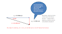
But, before we move on, let's take one last look at the velocity vectors that we were tracking previously.
Let's draw them at t = 3.6 seconds. (We're not confined to integers.)
We know that the horizontal velocity vx = 15.588 m/s. Always, for this particular projectile.
The vertical velocity was initially 9.000 m/s but it's changing at the rate of -3.711 m/s/s. After 3.6 seconds, it's been reduced by 3.711 m/s exactly 3.6 times. In terms of our models, vf = at + vi, so vf = (-3.711)3.6 + 9.000 = -4.360 m/s.
You should be able to add these vectors and determine the object's velocity, both magnitude and direction, at t = 3.6 s.
Click here for the answers, after working them out for yourself.
practice problems
additional resources

problems
*Excel file

instructions for video analysis using Logger Pro

save this video to your computer, open Logger Pro, then begin video analysis

This video is from a video game: Angry Birds.
You'll have to estimate their size to set your scale.
Then record and analyze your own video!


problems-
spot the error
*Excel file
I want to show you another way to analyze your data.
Take a look at the data tables below. To the standard three columns (t, x, and y), I have added additional columns to emphasize important patterns.
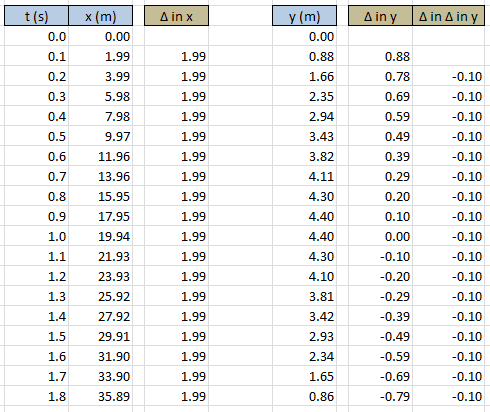
As long as our time interval remains constant, the change (∆) from one x-value (horizontal position) to the next remains constant. This implies a constant horizontal velocity, which we already expect for projectiles. (Note that the horizontal velocity is 19.9 m per second (m/s), not 1.99 m/s. In one second, we've moved forward 1.99 m a full ten times.)
Explicitly stated, the change in x over time is horizontal velocity. And it's constant for projectiles.
[In the language of calculus, the change of x over time is the derivative of x, with respect to time. That is, velocity is the time derivative of position.]
With regard to y, the change in position over time is not constant. The vertical velocity is not constant, which we already knew. Rather, the vertical velocity changes at a constant rate, defined as the acceleration, which is shown in the column ∆ in ∆ in y. (Note that the acceleration is not -0.10 m/s/s, because our time interval is not in seconds but tenths of a second. It is equivalent to -10.00 m/s/s, however, as we would expect on Earth (if we approximated).)
Explicitly stated, the rate (∆) at which the vertical velocity (∆ in y) changes is acceleration. And it, not the vertical velocity, is constant for projectiles.
[In the language of calculus, acceleration is the second time derivative of position and the first time derivative of velocity.]
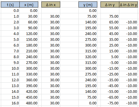
Here's another example for you to look over.
For this example, the time interval is 1.0 second. Thus, the horizontal velocity is simply 30.00 m/s and the vertical acceleration is -10.00 m/s/s.
now it's time for practice:

practice problem
*Excel file


Forces
Kinematics
